HYDROGEOLOGY
هیدروژئولوژی - مدل سازی و مدیریت آب زیرزمینیHYDROGEOLOGY
هیدروژئولوژی - مدل سازی و مدیریت آب زیرزمینیانتشار کتاب مدلسازی کاربردی جریان و انتقال جرم در آبخوان به همراه راهنمای نرم افزار GMS
امروزه مسئله برداشت بیش از حد از منابع آب زیرزمینی و آلوده شدن این آبها، به تهدیدی برای توسعه پایدار، حفظ امنیت غذایی و پیشرفت اقتصادی کشور ما تبدیل شده است. لذا ضرورت استفاده بهینه و حفاظت از آبخوانها، بیش از پیش احساس میشود. در این میان، مدلهای ریاضی ابزاری مفید و اقتصادی برای بررسی یک سیستم پیچیده آب زیرزمینی به شمار می آیند که امکان ارزیابی اثر اجرای سیاستهای مدیریتی بر یک آبخوان را فراهم می سازند.
با توجه به اینکه کتابهای بسیار کمی در زمینه مدلسازی آب زیرزمینی به زبان فارسی وجود دارند، تصمیم ما بر آن شد تا مجموعه ای شامل مبانی نظری مدلسازی جریان و انتقال آلاینده ها در آبخوان به همراه راهنمای کاربردی نرم افزار GMS- Groundwater Modeling System را در این کتاب گردآوری کنیم. این نرم افزار از جمله پیشرفته ترین و جامع ترین نرمافزارهای موجود میباشد و کاربران زیادی در ایران پیدا کرده است.
پژوهشگران و دانشجویان علاقهمند میتوانند برای خرید با شماره 09151012849 (مهندس رضا نظری) تماس گرفته و یا با ایمیل r.nazari10@gmail.com یا atajoodavi@gmail.com مکاتبه نمایند.
*قیمت: 15000 تومان
*در صورت خرید بیش از 3 جلد، ارسال از طریق پست رایگان می باشد.
*عرضه مستقیم کتاب در شهرهای مشهد و شیراز انجام میگیرد.
مقاله: چارچوب ایجاد مدل مفهومی
دانلود کتاب Applied groundwater modeling
Applied groundwater modeling
Mary P Anderson
***********************************************************
فصل نهم کتاب هیدرولوژی آب زیرزمینی تاد (مدل آب زیرزمینی)
***********************************************************
مراحل یادگیری مدل سازی آب زیرزمینی
با سلام. خیلی از دانشجویان از مراحل یادگیری مدل سازی آب زیرزمینی سوال کرده بودند. برای شروع مدل سازی ابتدا باید اطلاعاتی در مورد کد مادفلو داشته باشید. یکی از منابع فارسی موجود، کتاب "مدلسازی کاربردی جریان و انتقال آلاینده در آبخوان" و دیگری کتاب نون کرسیک است. همچنین می توانید از فصل نهم کتاب Todd استفاده کنید.
در مرحله بعدی باید کار کردن با نرم افزار GMS یاد بگیرید که بهترین روش استفاده از راهنمای خود نرم افزار است که بعد از نصب در این آدرس یافت می شود:
MyDocuments\GMS 7.1\Tutorials\
سپس راهنماها را به دقت و با ترتیب زیر مطالعه کنید:
ابتدا پوشه های Intro - GIS- Geostatistics.
بعد از آن از پوشه MODFLOW فایل های زیر را مطالعه کنید:
- MODFLOW-GridApproach
- MODFLOW-
ConceptualModelApproach - MODFLOW-ModelCalibration
- MODFLOW-
AutomatedParameterEstimation - MODFLOW-ManagingTransientData
لازم به ذکر است در اینجا حداقل اطلاعات لازم برای مطالعه ذکر شده است و برای مدل سازی پیشرفه نیاز به اطلاعات خیلی بیشتری می باشد.
- تعدادی از منابع مورد استفاده در مدل سازی آب زیرزمینی:
-
نظری، رضا، عطاءاله جودوی (1393)، مدلسازی کاربردی جریان و انتقال آلاینده در آبخوان. چاپ اول، نشر آفتاب عالمتاب، مشهد، 240 صفحه.
کرسیک، نون- ترجمه چیت سازان، منوچهر (1381). مدل سازی آبهای زیرزمینی، انتشارات دانشگاه شهید چمران اهواز.
-Thangarajan Regional, M. (2003). RegionalGroundwater Modeling.Capital Publishing Company.
-Batu, Vedat. (2006). Applied flow and solute transport modeling in aquifers. Taylor & Francis Group Inc.
-Harbaugh, A.W., Banta, E.R., Hill, M.C., and McDonald, M.G. (2000). MODFLOW-2000, User guide to modularization concepts and the ground-water flow process: U.S. Geological Survey Open-File Report 00-92, 121 p.
-Hill, Mary C. and Tiedeman, C. R. (2007). Effective groundwater model calibration. New Jersey: John Wiley & Sons, Inc
مقاله مدل سازی آب زیرزمینی دشت فیض آباد توسط نرم افزار GMS
برنامه ریزی منابع آب زیرزمینی در شرایط groundwater mining
مطالعه موردی: دشت فیض آباد
عطاءاله جودوی1- محمد زارع2
1دانشجوی دکتری آبشناسی، بخش علوم زمین، دانشگاه شیراز
2دانشیار گروه آبشناسی، بخش علوم زمین، دانشگاه شیراز
چکیده
توسعه بدون برنامه کشاورزی و برداشت بیش از حد از منابع آب زیرزمینی دشت فیض آباد (واقع در شمال شرق ایران) باعث بوجود آمدن شرایط groundwater mining و پیامدهای این موضوع مانند افزایش شوری آب زیرزمینی شده است. به علت اقلیم خشک این منطقه، بیشتر آب مصرفی در بخش کشاورزی از منابع آب زیرزمینی تامین می شود. به منظور برنامه ریزی منابع آب زیرزمینی، مدل جریان آب زیرزمینی دشت فیض آباد بوسیله MODFLOW تهیه شد. واسنجی مدل بواسطه انطباق بین سطح آب محاسباتی و مشاهده ای انجام شد و نتایج قابل قبولی بدست آمد. برای ارزیابی تأثیر برنامه فعلی بهره برداری و پیشنهاد کردن راه حل مناسب، چهار سناریوی مدیریتی تنظیم گردید و سناریوها بوسیله مدل مورد آزمایش واقع شدند. بر پایه نتایج مدل، بیلان شبیه سازی شده نشان داد برای متوقف کردن افت سطح آب زیرزمینی لازم است میزان برداشت ماهانه 40% کاهش یابد و در فصل زمستان بهره برداری از آب زیرزمینی صورت نگیرد.
در صورت نیاز به راهنمایی در مورد مدل سازی آب زیرزمینی، به این آدرس ایمیل بفرستید: atajoodavi@gmail.com
Steady State vs. Transient Modeling
Steady State vs. Transient Modeling
Groundwater flow models describe their capabilities as either steady state and/or transient. It is important when deciding upon groundwater modeling software to know which options are necessary for your needs. This month's newsletter will describe the key differences between steady state and transient modeling.
Steady state flow occurs when the magnitude and direction of flow is constant with time throughout the entire domain. Conversely, transient flow occurs when the magnitude and direction of the flow changes with time. In other words, the hydraulic head doesn't change with time in a steady state flow system, but does change during transient flow. This does not mean that in a steady state system there is no movement of groundwater, it simply means that the amount of water within the domain remains the same, and that the amount of water that flows into the system, is the same amount as flows out.
The steady state flow conditions simplify the groundwater flow equation significantly. When steady state flow occurs, time is no longer an independent variable and thus the storage term in the groundwater flow equation disappears; since there is no change in the amount of water within the domain (no change in hydraulic head) there is obviously no change in the amount of water stored in the domain.
References:
Fetter, C.Q. (1994). Applied Hydrogeology. Published by Maxwell Macmillan International, New York.
Freeze, R.A, and Cherry, J.A. (1979). Groundwater. Published by Prentice Hall, Inc., New Jersey.
MODFLOW
MODFLOW
Groundwater flow equation
- Kxx, Kyy and Kzz are the values of hydraulic conductivity along the x, y, and z coordinate axes (L/T)
- h is the potentiometric head (L)
- W is a volumetric flux per unit volume representing sources and/or sinks of water, where negative values are extractions, and positive values are injections (T−1)
- SS is the specific storage of the porous material (L−1); and
 is time (T)
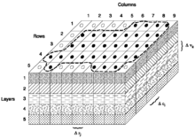
Finite difference

 is the hydraulic head at cell i,j,k at time step m
- CV, CR and CC are the hydraulic conductances, or branch conductances between node i,j,k and a neighboring node
 is the sum of coefficients of head from source and sink terms
 is the sum of constants from source and sink terms, where
  is flow out of the groundwater system (such as pumping) and
  is flow in (such as injection)
 is the specific storage
 ,
,  and
and 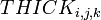 are the dimensions of cell i,j,k, which, when multiplied, represent the volume of the cell
 is the time at time step m
Limitations
- The water must have a constant density, dynamic viscosity (and consequently temperature) throughout the modelling domain (SEAWAT is a modified version of MODFLOW which is designed for density-dependent groundwater flow and transport)
 |
- The principle components of anisotropy of the hydraulic conductivity used in MODFLOW is displayed on the right. This tensor does not allow non-orthogonal anisotropies, as could be expected from flow in fractures. Horizontal anisotropy for an entire layer can be represented by the coefficient "TRPY" (Data Item 3 Page 153 [2].
Computer codes for GROUNDWATER MODELING
Computer Codes
- MODFLOW
- MODFLOWP (Hill, 1992).
- MOC3D (Three-DimensionalMethod-of-Characteristics Ground-Water Flow and Transport Model).
- MT3DMS (Modular 3-D Multi-Species Transport Model for Simulation of Advection, Dispersion, and Chemical Reactions of Contaminants in Groundwater Systems).
- RT3D (Multi-Species Reactive Flow and Transport Simulation Software).
- HST3D (Heat and Solute Transport in Three-Dimensional Groundwater Systems).
- FEMWATER (Three-Dimensional Finite Element Model of Water Flow Through Saturated-Unsaturated Media).
- Random-Walk (Random-Walk Solute TransportModel for Selected Groundwater Quality Evaluations).
- GMS (Groundwater Modeling System). GMS is a software pre-processor, post-processor, and graphic user interface (GUI) implementation of a number of public domain groundwater modeling computer codes, which include FEMWATER, MODFLOW, MODPATH, MT3DMS, RT3D, UTCHEM, and PEST. It was developed by the U.S. Army Engineer Research and Development Center for use by governmental agencies. It is available as a commercial software.
- SWAT (Soil and Water Assessment Tool). SWAT (Arnold and Fohrer, 2005; Neitsch et al., 2005) is a basin scale, continuous time model designed to predict the impact of management on water, sediments, and agricultural chemical yields in ungaged watersheds. Major model components include weather, hydrology, soil temperature and properties, plant growth, nutrients, pesticides, bacteria and pathogens, and land management. In SWAT, a watershed is divided into multiple sub-watersheds, which are then further subdivided into hydrologic response units that consist of homogeneous land use, management, and soil characteristics. SWAT is a public domain code supported by the U.S.D.A. Agricultural Research Service at the Grassland, Soil and Water Research Laboratory.
- HYDRUS (Movement of Water, Heat, and Multiple Solutes in Variably Saturated Media).
- FEFLOW (Finite Element Subsurface Flow and Transport Simulation System).
- PEST (Model-independent parameter estimation).
- SUTRA (Model for 2D or 3D Saturated-Unsaturated, Variable-Density Ground-Water Flow, with Solute or Energy Transport).
- SEAWAT (Computer Programfor Simulation of Three-Dimensional Variable-Density Ground-Water Flow).
- CODESA-3D (Coupled Variable Density and Saturation 3D Model).
- SHARP (A Quasi-Three-Dimensional, Numerical FDMthat Simulates Freshwater and Saltwater Flow Separated by a Sharp Interface in a Layered Coastal Aquifer Systems).
- ParFlow (Modeling Surface and Subsurface Flow on High Performance Computers).
- TOUGH (Transport of Unsaturated Groundwater and Heat).
- NUFT (Nonisothermal, Unsaturated Flow and Transport with Chemistry).
- STOMP (Subsurface Transport Over Multiple Phases).
- SLAEM/MLAEM (Single/Multi-Layer Analytic Element Method).
- WHPA (Wellhead Protection Area).
- BIOPLUME. BIOPLUME is a two-dimensional computer code for simulating contaminant transport of a single and multiple hydrocarbons with oxygen-limited and reactant-limited bioreactions (Rafai et al., 1998), developed by EPA. Its transport code is based on the USGS MOC.
- NAPL Simulator. The NAPL Simulator is an EPA three-dimensional computer code based on Hermite collocation finite element discretization (Guarnaccia et al., 1997).
- UTCHEM (University of Texas Chemical Compositional Simulator). Originally a three-dimensional finite difference model for multiphase flow, multicomponent transport and chemical flooding, this code has been modified to become a general purpose NAPL simulator (University of Texas, 2000).
- BIOMOC (A Multispecies Solute-Transport Model with Biodegradation).
- PHREEQC (A Computer Program for Speciation, Batch-Reaction, One-Dimensional Transport, and Inverse Geochemical Calculations).
- PHAST (Program for Simulating Ground-Water Flow, Solute Transport, and Multicomponent Geochemical Reactions).
Source: Bear, Jacob, Cheng, Alexander (2010), Modeling Groundwater Flow and Contaminant Transport.