HYDROGEOLOGY

Steady State vs. Transient Modeling

Groundwater flow models describe their capabilities as either steady state and/or transient. It is important when deciding upon groundwater modeling software to know which options are necessary for your needs. This month's newsletter will describe the key differences between steady state and transient modeling.

Steady state flow occurs when the magnitude and direction of flow is constant with time throughout the entire domain. Conversely, transient flow occurs when the magnitude and direction of the flow changes with time. In other words, the hydraulic head doesn't change with time in a steady state flow system, but does change during transient flow. This does not mean that in a steady state system there is no movement of groundwater, it simply means that the amount of water within the domain remains the same, and that the amount of water that flows into the system, is the same amount as flows out.

The steady state flow conditions simplify the groundwater flow equation significantly. When steady state flow occurs, time is no longer an independent variable and thus the storage term in the groundwater flow equation disappears; since there is no change in the amount of water within the domain (no change in hydraulic head) there is obviously no change in the amount of water stored in the domain.

References:

Fetter, C.Q. (1994). Applied Hydrogeology. Published by Maxwell Macmillan International, New York.

Freeze, R.A, and Cherry, J.A. (1979). Groundwater. Published by Prentice Hall, Inc., New Jersey.

عطاءاله جودوی 24 خرداد 1390 ساعت 00:29

0 نظر

MODFLOW

MODFLOW is the U.S. Geological Survey modular finite-difference flow model, which is a computer code that solves the groundwater flow equation. The program is used by hydrogeologists to simulate the flow of groundwater through aquifers. The code is free software, written primarily in Fortran, and can compile and run on DOS, Windows or Unix-like operating systems.

3-dimensional grid

Since its original development in the early 1980s,the USGS have released four major releases, and is now considered to be the de facto standard code for aquifer simulation. Currently, there are at least five actively developed commercial and non-commercial graphical user interfaces for MODFLOW.

Groundwater flow equation

The governing partial differential equation used in MODFLOW is:

$\frac{\partial}{\partial x} \left[ K_{xx} \frac{\partial h}{\partial x} \right] + \frac{\partial}{\partial y} \left[ K_{yy} \frac{\partial h}{\partial y} \right] + \frac{\partial}{\partial z} \left[ K_{zz} \frac{\partial h}{\partial z} \right] + W = S_{S} \frac{\partial h}{\partial t}$

where

$K x x$ , $K y y$ and $K z z$ are the values of hydraulic conductivity along the x, y, and z coordinate axes (L/T)
$h$ is the potentiometric head (L)
$W$ is a volumetric flux per unit volume representing sources and/or sinks of water, where negative values are extractions, and positive values are injections (T⁻¹)
$S S$ is the specific storage of the porous material (L⁻¹); and
$t\,$ is time (T)

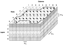
Finite difference

The finite difference form of the partial differential in a discretized aquifer domain (represented using rows, columns and layers) is:

$\begin{align} & CR_{i,j-\tfrac{1}{2},k}\left(h^m_{i,j-1,k}-h^m_{i,j,k}\right) + CR_{i,j+\tfrac{1}{2},k}\left(h^m_{i,j+1,k}-h^m_{i,j,k}\right) + \\ & CC_{i-\tfrac{1}{2},j,k}\left(h^m_{i-1,j,k}-h^m_{i,j,k}\right) + CC_{i+\tfrac{1}{2},j,k}\left(h^m_{i+1,j,k}-h^m_{i,j,k}\right) + \\ & CV_{i,j,k-\tfrac{1}{2}}\left(h^m_{i,j,k-1}-h^m_{i,j,k}\right) + CV_{i,j,k+\tfrac{1}{2}}\left(h^m_{i,j,k+1}-h^m_{i,j,k}\right) + \\ & P_{i,j,k}\,h^m_{i,j,k} + Q_{i,j,k} = SS_{i,j,k}\left(DELR_j \cdot DELC_i \cdot THICK_{i,j,k}\right) \frac{h^m_{i,j,k}-h^{m-1}_{i,j,k}}{t^m-t^{m-1}} \end{align}$

where

$h^m_{i,j,k}\,$ is the hydraulic head at cell i,j,k at time step m
CV, CR and CC are the hydraulic conductances, or branch conductances between node i,j,k and a neighboring node
$P_{i,j,k}\,$ is the sum of coefficients of head from source and sink terms
$Q_{i,j,k}\,$ is the sum of constants from source and sink terms, where $Q_{i,j,k}<0.0\,$ is flow out of the groundwater system (such as pumping) and $Q_{i,j,k}>0.0\,$ is flow in (such as injection)
$SS_{i,j,k}\,$ is the specific storage
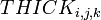$DELR_j\,$ , $DELC_i\,$ and $THICK_{i,j,k}\,$ are the dimensions of cell i,j,k, which, when multiplied, represent the volume of the cell
$t^m\,$ is the time at time step m

Limitations

The water must have a constant density, dynamic viscosity (and consequently temperature) throughout the modelling domain (SEAWAT is a modified version of MODFLOW which is designed for density-dependent groundwater flow and transport)

$\mathbf{K} = \begin{bmatrix} K_{xx} & 0 & 0 \\ 0 & K_{yy} & 0 \\ 0 & 0 & K_{zz}\end{bmatrix} \$

The principle components of anisotropy of the hydraulic conductivity used in MODFLOW is displayed on the right. This tensor does not allow non-orthogonal anisotropies, as could be expected from flow in fractures. Horizontal anisotropy for an entire layer can be represented by the coefficient "TRPY" (Data Item 3 Page 153 ^[2].

عطاءاله جودوی 24 خرداد 1390 ساعت 00:28

0 نظر

Computer codes for GROUNDWATER MODELING

Computer Codes

MODFLOW
MODFLOWP (Hill, 1992).
MOC3D (Three-DimensionalMethod-of-Characteristics Ground-Water Flow and Transport Model).
MT3DMS (Modular 3-D Multi-Species Transport Model for Simulation of Advection, Dispersion, and Chemical Reactions of Contaminants in Groundwater Systems).
RT3D (Multi-Species Reactive Flow and Transport Simulation Software).
HST3D (Heat and Solute Transport in Three-Dimensional Groundwater Systems).
FEMWATER (Three-Dimensional Finite Element Model of Water Flow Through Saturated-Unsaturated Media).
Random-Walk (Random-Walk Solute TransportModel for Selected Groundwater Quality Evaluations).
GMS (Groundwater Modeling System). GMS is a software pre-processor, post-processor, and graphic user interface (GUI) implementation of a number of public domain groundwater modeling computer codes, which include FEMWATER, MODFLOW, MODPATH, MT3DMS, RT3D, UTCHEM, and PEST. It was developed by the U.S. Army Engineer Research and Development Center for use by governmental agencies. It is available as a commercial software.
SWAT (Soil and Water Assessment Tool). SWAT (Arnold and Fohrer, 2005; Neitsch et al., 2005) is a basin scale, continuous time model designed to predict the impact of management on water, sediments, and agricultural chemical yields in ungaged watersheds. Major model components include weather, hydrology, soil temperature and properties, plant growth, nutrients, pesticides, bacteria and pathogens, and land management. In SWAT, a watershed is divided into multiple sub-watersheds, which are then further subdivided into hydrologic response units that consist of homogeneous land use, management, and soil characteristics. SWAT is a public domain code supported by the U.S.D.A. Agricultural Research Service at the Grassland, Soil and Water Research Laboratory.
HYDRUS (Movement of Water, Heat, and Multiple Solutes in Variably Saturated Media).
FEFLOW (Finite Element Subsurface Flow and Transport Simulation System).
PEST (Model-independent parameter estimation).
SUTRA (Model for 2D or 3D Saturated-Unsaturated, Variable-Density Ground-Water Flow, with Solute or Energy Transport).
SEAWAT (Computer Programfor Simulation of Three-Dimensional Variable-Density Ground-Water Flow).
CODESA-3D (Coupled Variable Density and Saturation 3D Model).
SHARP (A Quasi-Three-Dimensional, Numerical FDMthat Simulates Freshwater and Saltwater Flow Separated by a Sharp Interface in a Layered Coastal Aquifer Systems).
ParFlow (Modeling Surface and Subsurface Flow on High Performance Computers).
TOUGH (Transport of Unsaturated Groundwater and Heat).
NUFT (Nonisothermal, Unsaturated Flow and Transport with Chemistry).
STOMP (Subsurface Transport Over Multiple Phases).
SLAEM/MLAEM (Single/Multi-Layer Analytic Element Method).
WHPA (Wellhead Protection Area).
BIOPLUME. BIOPLUME is a two-dimensional computer code for simulating contaminant transport of a single and multiple hydrocarbons with oxygen-limited and reactant-limited bioreactions (Rafai et al., 1998), developed by EPA. Its transport code is based on the USGS MOC.
NAPL Simulator. The NAPL Simulator is an EPA three-dimensional computer code based on Hermite collocation finite element discretization (Guarnaccia et al., 1997).
UTCHEM (University of Texas Chemical Compositional Simulator). Originally a three-dimensional finite difference model for multiphase flow, multicomponent transport and chemical flooding, this code has been modified to become a general purpose NAPL simulator (University of Texas, 2000).
BIOMOC (A Multispecies Solute-Transport Model with Biodegradation).
PHREEQC (A Computer Program for Speciation, Batch-Reaction, One-Dimensional Transport, and Inverse Geochemical Calculations).
PHAST (Program for Simulating Ground-Water Flow, Solute Transport, and Multicomponent Geochemical Reactions).

Source: Bear, Jacob, Cheng, Alexander (2010), Modeling Groundwater Flow and Contaminant Transport.

عطاءاله جودوی 24 خرداد 1390 ساعت 00:25

0 نظر

HYDROGEOLOGY

HYDROGEOLOGY

درباره من

تقویم

Steady State vs. Transient Modeling

MODFLOW

MODFLOW